

Harley E. A. Bicas
DOI: 10.17545/eOftalmo/2021.0012
ABSTRACT
Refraction from elliptical surface sections is analyzed in this study. With specific adjustments of their eccentricities, the condition of aspherical refraction (image formation at an only point the focal point of the surface can be achieved when the incident wave exhibits plane wavefronts and propagates parallel to the optical axis, i.e., when the object (radiant power source) is at infinite distance. On the contrary, for objects located at finite distances, elliptical surfaces cannot produce aspherical refraction. The formulations and their respective demonstrative calculations are presented in this study. We also show that multifocality, governed by varying radii of curvature on a surface, is a specific optical condition of elliptical sections which serve as matrices of these refractometric applications.
Keywords: Aspherical refraction; Elliptical surfaces; Multifocality.
RESUMO
Considera-se a refração em secções de superfícies elípticas para mostrar que com ajustamentos específicos de suas excentricidades se possa prover a condição de “asfericidade” (formação da imagem em um único ponto, o foco imagem da superfície) quando a incidência for a de frentes de ondas planas e com direção paralela ao eixo óptico, isto é, quando o objeto (fonte de energia radiante) estiver à distância infinita. Contrariamente, para objetos situados a distâncias finitas, a “asfericidade” não pode ser assegurada por superfícies elípticas. As formulações e os respectivos cálculos demonstrativos são apresentados. Também se mostra que a multifocalidade, dependente de raios de curvatura variáveis em uma superfície, é condição óptica própria das secções elípticas que servem como matrizes dessas aplicações refratométricas.
Palavras-chave: Refração esférica; Superfícies elípticas; Multifocalidade.
INTRODUCTION
The study of optical geometry is of paramount importance in ophthalmology, since it addresses one of the most commonly used aspects in its daily practice: eye refractometry with its possible resulting applications (prescription of optical corrections). In fact, it is recognized that eye consultations, for the most part, occur due to problems that can be corrected by the proper application of simple measures related to eye refraction, such as eyeglass, contact, and intraocular lenses; surgical remodeling of the anterior face of the cornea; and other interventions. Thus, in the two most important books published by the Brazilian Council of Ophthalmology on the subject, the emphasis given to the optical phenomenon of refraction and its applications, in the first sentence of their prefaces, is paradigmatic. The oldest one1 starts by quoting that “Eye refractometry is the most demanding procedure among all who take a person to eye consultation.” The more recent book2 reiterates this importance in the following: “Among the multiple actions expected of an ophthalmologist in the exercise of his profession, the most common is optical prescriptions.”
Obviously, knowledge about refraction is not limited to such specialists. It extends to those who develop the principles for these solutions as well as to those who manufacture or sell the products that make them possible. This knowledge is also valuable for other diverse areas of human activity, such as visual prospection of far distant objects (astronomical or terrestrial telescopy) or those very small (microscopy). In fact, until recently, refraction was regarded as an optical phenomenon linked to the propagation of visible light. Currently, however, refraction is known to be more general, extending to radiations of any frequency.
Despite not being an exclusively optical phenomenon, refraction was first described in such connotation. In fact, the empirical observations obtained in the 2nd century by Ptolemy (Klaúdius Ptolemaios who lived from 90-168 AC according to some sources, or 100-160 AC according to others) are surprising. His measurements of refractive angles from air to water and air to glass, are remarkable approximations of the exact values, especially considering the relatively precarious instrumentation he used to obtain those results. For example, for every 10° increments from 0° to 60°, from air to water, his absolute errors are between 0 to 39’ (at the incidence of 20°), (16.14’±16.48’).From air to glass, the errors were between 0 to 34’ (at the incidence of 20°), (17.12±15.11) , with an overall average error margin of only 2.08%. Almost all differences are accounted by the fact that measured values exceed the real exact values, which we could attribute to a systematic error in the measurement process. It is therefore quite possible that if Ptolemy had the mathematical arsenal by which the law of refraction was later enunciated, he would have come to its formulation. He correctly postulated that when light (or rays of vision) penetrate a medium with a higher refractive index, it approaches the perpendicular to the surface; contrarily, when it travels from that medium to another medium possessing a lower refractive index (air), it distances itself from that perpendicular (Hirschberg, p. 151)3, a principle that remains unchanged.
It took another millennium and a half since then for the generic law of refraction-a concept with elegant simplicity-to be formulated once the mathematical instrumental necessary to enunciate this knowledge was unveiled in the 17th century. It addresses the possible change of direction of propagation of radiant energy on a medium toward that of the refracted radiant energy in the next, at each specific point of a surface separating them.
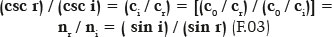
This discovery is attributed to Willebrord Snel van Royen (1580-1626), or Willebrord Snellius (with two “l”s in the Latin transcription of his Dutch name, due to which the Anglo-Saxon version of his name “Snell” became widespread). Without a specific date to certify it (being discovered only after his death) Snell wrote the following:

where the cosecants of the incidence (csc i) and refraction (csc r) angles are inversely proportional to the speeds of light in their respective media (ci or cr). The canonical form, as it is now known, was proposed by René Descartes (1637) :

where the sine of the incidence (sin i) and refractive (sin r) angles are inversely proportional to the refractive indices of their respective mediums. The refractive index of a medium (such as that of incidence, ni) corresponds to the speed of light value in that medium (such as that of incidence, ci) relative to the speed of light in vacuum (c0), i.e., ni = c0/ ci. Therefore, a value of inverse magnitude, implying a lower speed of light in the medium, results in a higher refractive index. Given that the cosecant of an angle is the reciprocal trigonometric function of the respective sine and considering the refractive index is the reciprocal of the speed of light, there is an absolute reciprocity between the formulations of Snell and Descartes, which substantiates using the expression “Snell-Descartes” law:
The phenomenon of refraction, therefore, is governed by a principle formulated using the relationship of angles (expressed by a trigonometric function), which is universally reproducible for the pair of mediums between which it occurs, i.e., the relationship between its refraction indices remains constant. Quantifying these angles of incidence, i, and of refraction, r, implicitly requires the establishment of a reference, which is the imaginary normal line or the perpendicular to the point where refraction occurs.
In geometry, perpendicular lines to a point is nonsensical (infinite straight lines in any directions can pass through a point). To solve this question, one considers that the point where the refraction occurs is the place where, both, the surface (which has the point) and a tangent to it coincide. So that, a perpendicular to the tangent surface at this point is also perpendicular to the surface at that point. In other words, among the infinite lines which could serve as reference, only one, the “normal line” to the surface is valid. Therefore, although refraction is, effectively, a punctual phenomenon, it depends on the curvature of the surface at the point where it occurs.In other words, the claim that refraction at a point is independent of the surface is only partially correct. In its essence, the assertion is true: a light ray’s direction (direction of the wave front with which radiant energy is propagated) remains the same regardless of whether the surface is flat, concave, convex, or in any other shape (Figure 1). However, this statement does not apply to one of the main practical applications of optics, in determining the image position of an object (Figure 1).
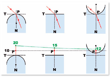
E.g.: for an object (P) located at distance p= -10 cm, if we assume the radii of curvature for the convex (R= +20 cm), flat (R= +∞), and concave (R = -20) surfaces, their respective images will form at distances q = -20, -15 and -12 cm, i.e., in different positions relative to each of the surfaces, dependent on the respective surface curvatures at the point considered. If the object was at -100 cm, the positions of the images are +100, -150 and -42.86 cm respectively.
Curvature of a surface
Although refraction is postulated as occurring at a “point”, the correct claim is that it shall be measured relatively to a perpendicular line to it. Which refers to either a surface, a section of it (in three-dimensional space), or to another (tangent) line (in two-dimensional space). In other words, the treatment of a perpendicular to a point on a surface (or line) is subjected to the geometry of a surface’s curvature (or line) at that specific point, and this perpendicular is quantified by the radius of curvature of a surface (or line) at that specific point. Essentially, the concept of refraction is closely dependent on a surface’s (or line’s) curvature at one of its points.
Lines or surfaces may be mathematically defined by their curvatures, or by their reciprocal curvature radii: either constant and infinite (that of a straight line, or a plane), constant and finite (those of circles, or spheres), or progressively variables (e.g., those of conical sections, spheroids, or ellipsoids ), among other natures. Refraction on flat surfaces has been widely studied in optical prisms. On the other hand, ophthalmic lenses for correcting ocular optical defects are all curved (one of their faces, at least). Nevertheless, it is odd that their refraction principles may be explained simply by the principles of spherical surfaces (given the relative simplicity of their geometry). Moreover, although it is recognized that the study of spherical optics is inherently defective, given the spherical aberration phenomenon,the approach of alternative curves is not commonly offered. But elliptical surface optics would provide the solutions to aspherical lens optics (that is, without presenting spherical aberration) and optical refinements as those of multifocal lenses.
In fact, a thorough study of curvatures imposes great difficulties such as requiring knowledge of differential geometry. In certain simpler cases, such as refraction on elliptical surfaces, the Cartesian analytical treatment of problems would suffice. Even so, the discomfort of following these paths is notorious, as wisely exposed in the presentation of another highly celebrated national textbook4, alluding to an undeniable pedagogical reference on the study of refraction5: “fortunately Donders was self-admittedly no mathematician and he wrote in clear and simple language, so that his book became popular.” And also, in subsequent complementation, the author of another classic work6, “Duke-Elder’s Practice of Refraction” (1st Edition 1928), sought to avoid a mathematical presentation of refraction errors and the way to correct them4.
Unequivocally, mathematical developments are generally difficult to follow up when they are unfamiliar, but indispensable to those who want to deepen any subject on which they are founded (the celebrated Helmholtz, in his celebrated three volumes of the Treaty on Physiological Optics, overused this resource). This does not justify the lack of reference to the nature of the solution of the problem. The lack of any mention of terms such as “ellipse” and “elliptical curve (or surface)” or similar terms is absolutely disconcerting, as is any correlation to the optics presented either in books on the study of refraction-those discussed earlier1-6, others7-10, those dedicated to optics (lenses manufacture)11,12, or even in the most well-known international literature-old and recent alike 13-25. When used, these terms have little in common with the refraction phenomenon’s own nature; e.g., the Tscherning ellipse24 (a graphical expression of the relationship between the dioptric power of ophthalmic lenses and the recommended base curves), or elliptical polarization19 (in relation to one of the modalities of the electromagnetic energy polarization phenomenon). In fact, even when elliptical sections are considered, such as sections of cylindrical (or toric) lenses inclined relative to their axes, the optics of elliptical sections are not described . In fact, one of the most important ophthalmological compendiums26 states that “The surface dealt with in optics are generally spherical in shape ... while the production of non-spherical or asphericsurfaces (which are actually more desirable in some instances) is extremely difficult. For this reason, spherical surfaces are employed almost exclusively in optics, and they usually perform adequately” (pp. 6-7)26. Even when addressing cylindrical lenses, no reference is made to “ellipticals” (for their sections) On the contrary, little familiarity with such elementary geometric issues leads to the surprising statement that “There is no optical power in oblique meridians of a toric refracting surface” (p. 46, op. cit.). The mistake was not to consider the coplanarity of the incident and refracted rays, but to consider “...’skew rays’ because they are skewed about the axis,” with which the text concludes as follows: “these limiting rays are deviated by different amounts in the two corresponding directions” (The bold type was my addition). In a later edition27 this oversight is corrected, acknowledging that “There is a different power in every meridian” (p. 87), which is illustrated by an enlightening figure (fig. 72), despite it not detailing how and why this refraction (on elliptical surfaces) may occur.
In the revered and deep treatise on physiological optics by Helmholtz, there is a reference to “ellipsoidal refracting surface” (volume I, p. 194)13, but its content is subject to aberrations occurring in refraction by the surface of an ellipsoid (such as that of an astigmatic cornea), describing the geometric figure that is modernly known as the “Sturm’s Conoid.” In fact, Helmholtz duly credits this author in the previous chapter of the same volume, although followed by a corrective remark14: “Aberrations of the kind that Sturm supposes actually do seem to occur in most human eyes, and the phenomena dependent on them will be described; where, however, it will be shown that the interval between the two focal planes is by no means so important as STURM thinks and that, instead of promoting the clearness of vision, this defect in the eye tends rather to impair it.” It should be noted that even Allvar Gullstrand-who was awarded the Nobel Prize in Physiology or Medicine in 1911, precisely for his studies on ocular dioptrics-invited to review this monumental work by Helmholtz and to enrich it with the insertion of his perspicacious notes and appendices, does not dwell on the subject, nor does it mention ellipses and their optics28.
In short, the lack of explicit references to refraction on elliptical surfaces appears to justify its’ succinct presentation, in order to eventually arouse interests in its’ further deepening.
Refraction by spherical surfaces
Spheres offer great simplicity in the study of refraction, given their curvature remains constant at any point, i.e., a single center through which all normal lines pass, which are also perpendicular to any tangents of its surface. The flat sections of a sphere are circles with different radii of curvature, the maximum value of which corresponds to that of the equatorial diameter.
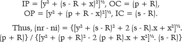
The fact that there exists only one center (C) allows relative measurement of its radius of curvature (R) from its surface and the distances from the center to an object point (p) and that to its respective image, as a function of the angle of incidence (i). Note that because one considers a point object, regardless of its position in space relative to the spherical surface, the object can always be considered to be on the same line that contains its center of curvature, i.e., on a respective optical axis. Figure 2 shows that applying the law of sines to OPC and CIP triangles respectively results in
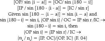
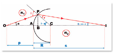
This geometric representation (F. 04) can be transformed into the variables of their respective meanings, i.e., the distances p, s, and R and the coordinates of point P, since
From the equation of circles, x2 + y2 = R2; thus,
i.e., given the values of the variables y (point of incidence “height,” relative to the optical axis) and R (radius of a surface’s curvature), a second-degree equation can be derived to calculate s (depending on p), or of p (as a function of s).
In any case, this formulation, although generic, is avoided. Instead, the paraxial ray equation is preferred, which implies a negligible incidence angle value (incidence “coincident” to the optical axis). In fact, if y = 0,
Even more common is the formula resulting from a development of the above.
An F-value is a surface’s focal power and is expressed in the optical unit diopters (with the symbol D) when the radius of curvature (R) is quantified in meters. It is constant for each spherical surface for it depends on invariable values: the radius of curvature of the surface (R) and the refractive indices of the media separated by it (ni, of the incidence medium, and nr , of the refractive medium).
Another simplification of the generic formula (F. 05) is to consider an object’s position at an infinite distance. Hence,
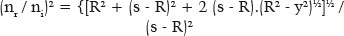
a quadratic equation for the value (s − R), dependent on the variable y. Solving the second-degree equation:
In this case, y = R sin i:
This formula is very important because it shows that rays parallel to the optical axis (i.e., effectively coming from an infinite distance) reach the surface at different heights relative to the optical axis (y) and, or, with different values of the angle of incidence (i), will produce images at different distances (s) from the surface, that is, a longitudinal spherical aberration. For example, table 1 shows that s values depend on those of y, for nr = 1.5, ni = 1.0, R = 20 cm.
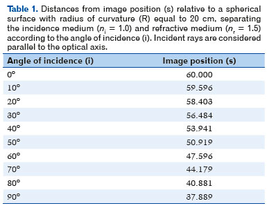
In other words, energy reaching a surface does not concentrate on a single point (focus) but rather disperses over a space whose boundaries are contained by a surface called caustic (Figure 3).
Aspherical surfaces
The undesirable condition of spherical aberration makes it desirable to seek another surface that can concentrate refracted energy at a single point (the image focal point, that of the image distance of an object situated on the optical axis and infinite distance; s = 60 cm Table 1 example), all the energy incident on the surface. This is equivalent to searching for surfaces whose radii of curvature are progressively larger, i.e., less sharp curvatures. In other words, determining the specific radius of curvature (Ry) for each height relative to the optical axis (y) could enable the image of the object to coincide with the image corresponding to the incidence i = 0°.
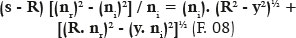
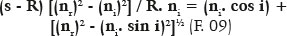
Therefore, it boils down to rearranging the same F. 09, but by switching the sought variable, which is the value of the curvature radius (Ry) such that the image position is always the same (s = 60 cm, Table 2). To facilitate the calculation of R according to the other variables, F. 09 must be rearranged to
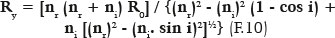
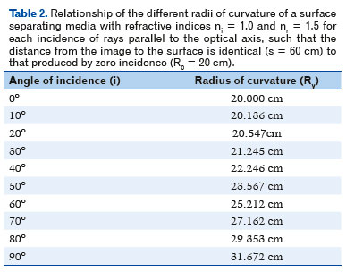
Figure 4 illustrates tables 1 and 2, which show the variation of an image’s position according to the height relative to the optical axis in which the incidence of a radius is parallel to it (Figure 4A); further, it conversely shows the curvature radius variation required for an image to always form on the same point (Figure 4B).
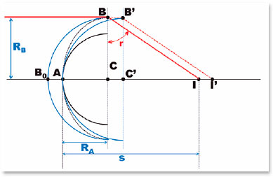
The underlying principle of table 2 raises some remarks, as explained in figure 5. In fact, the distance at which the image of a null incidence (i = 0°) formed by the surface with center C and radius of curvature AC = RA is formed is AI = s. A surface with a greater radius of curvature, RB = BC, with the same center of surface A, forms the image for incidence i = 90° at the same location (I). However, for this to occur, its apex (the position in which the surface is cut by the optical axis) must be at B0, a place which does not coincide with that of the apex of the anterior surface that generated the first image (A). If there these apices coincided (in A), the curve of that surface would describe arc AB’, its center of curvature would not be C, but C’ and the position of the image would be at I’ (Figure 5). Thus, in order for the apices to coincide (at A), as much as the centers of curvature (at C), the drawing of curves with images formed in the same location (I), without the so-called “spherical aberration,” must follow another curve (line interrupted between A and B in Figure 5).
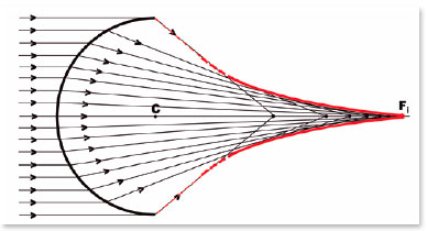
In fact, there are several curves with increasing or decreasing progressions of the curvature radii at each of its points. Ellipses are those that enable the adjustment of refractive variables (refractive indices between the media separated by the surface and variable radii of curvature) such that refracted rays are always formed at the same “focal” point (Figure 6).
In fact, unlike spherical surfaces in which refraction aberration appears, precisely because of their constant radius of curvature, on elliptical surfaces an increasing or decreasing progression of these radii of curvature can be observed (Figure 7), determining either an accentuation of those aberrations, or their reduction until they are canceled and reverted. Thus, a single specific shape (for each pair of optical medium separated by the surface) is the one that relates to the condition of non-aberration of sphericity, although strictly speaking, all of them are aspherical, that is, non spherical (Figure 8).
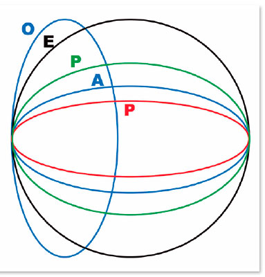
One of the distinctive mathematical traits of the ellipses is their eccentricity-a value that corresponds to their deformation relative to the circle. (The circle’s eccentricity is zero.) However, the eccentricity of an ellipse cannot be directly associated with an aberration type, since the same ellipse (thus, the same eccentricity) can relate to the optical axis in several ways. In fact, ellipses O and A (Figures 7 and 8) are identical in their eccentricities, but differ when relating to the optical axis, with the longest of their axes in the horizontal plane (curve A) or to the smallest (curve O), which effects on refraction are completely different. Note that the inverse occurs for the curvature radius of the horizontal apical point: the shortest curvature radius is that of curve A and the longest is that of O.
The semantic issue of asphericity
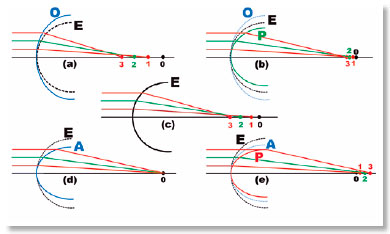
Obviously, whether by increasing or decreasing variations of the curvature radii, all resulting curves are “non-spherical”, or “aspherical”.All curves produce refractional aberration by the surface’s shape, with the exception of one. This special optical surface is termed as “non-aberrant” or “inaberrant.” Thus, the most appropriate terminologies to define the type of aberration are superaberration (positive) when this aberration is increased with respect to spherical aberration (curve O, Figure 8a), subaberration when it is reduced (P, Figure 8b), simply “inaberration” when there is no aberration (curve A, Figure 8d), and contraberration (negative) when it reverses direction (curve P, Figure 8e). Oblate curves are always superaberrant, whereas prolates may be subaberrant (Figure 8b), inaberrant (Figure 8d), or contraberrant (Figure 8e). There is therefore no reason to say that inaberrant surfaces are prolate, for despite this being true, it represents a particular case: not every prolate curve is inaberrant.
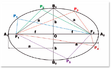
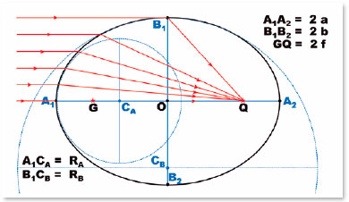
The geometry of ellipses
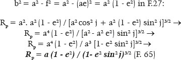
Other elements of the ellipse geometry are not shown in figure 9, but in figure 10. In ellipses, because the distance between B1 (or B2) and one of the foci (G or Q) equals the length of the major semiaxis (a), the following relationship between variables a, b, and f becomes evident:
The ellipse’s canonical equation, which relates the Cartesian coordinates of one of its points P(x, y) in relation to the origin of the measurement system (simplifiedly taken as the center of the ellipse), can be deduced from figure 9’s elements as follows:

Another relationship is the one defining the ellipse’s eccentricity (e):
This value (of eccentricity, e) distinguishes the so-called conical sections, namely
(a) The circle (e = 0) obtained by the flat section of the cone perpendicular to its main axis.
b) The ellipses (1 > e > 0) obtained by the flat section of the cone inclined relative to its main axis but crossing it.
c) The parabola (e = 1) obtained by the flat section of the cone, parallel to one of its geratrices (lines connecting the apex to the base).
d) The hyperbolas (e > 1) obtained by the flat section of the cone, parallel, or inclined to its main axis, but without crossing it.
The relationship of the Cartesian coordinates of a point P (x, y) in a system which origin is the center of the O ellipse (0.0) is given by
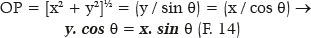
By replacing y of F. 14 in the canonical ellipse equation (F. 12), we get
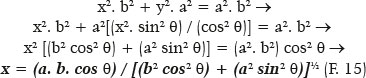
Similarly,

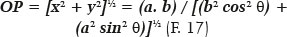
Therefore, the distance from the point (P) to the ellipse’s center (O), i.e., the OP distance is given by
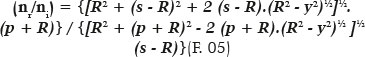
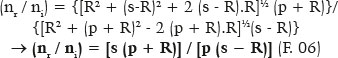
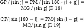
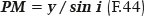
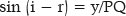
A very important condition is that the normal at each point of the ellipse (i.e., the line perpendicular to the tangent of the ellipse at that point) is the bisector of the angle between the lines between it (P, Figure 10) and the foci of the ellipse (G and Q). That line (PM, Figure 10) defines angular relationships (j and g, in the GPM triangle), by which the angle of incidence (i) and the angle of refraction (r) at a point on the surface will then be considered.
Consequently, relationships can be established for the GPM and MPQ triangles:
A number of developments may originate henceforth. Note that
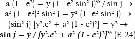
Let us consider the values of GM and MQ from F. 18 and F. 19, respectively:
The (1 - e2) = k set can be useful to simplify equations, as shown next. In any case, F. 23 gives the value of j according to that of PM (or vice versa). Given sin j = y / PM, then
and therefore,

Equation F. 17 (and similarly, F. 15 and F. 16) can be rewritten as a function of k = 1 - e2 :
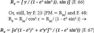
The equation for the radius of curvature at one of the points P on the surface (RP) is

which leads to the conclusion that for one of the vertices of the major axis (j = 0°),

whereas for one of the vertices of the minor axis (j = 90°),

The location of the curvature’s center in relation to each of the points on the surface will be considered later; nevertheless, the relationships on the refraction of a curve without spherical aberration can be exemplified.
Refraction on a surface without spherical aberration
Consider an object point located at an infinite distance from a surface that separates two media, those of the incidence and of the refraction, with refractive indices ni and nr, respectively (nr > ni). Consider “A” a point on this surface where the incident radiation occurs and let q be a finite distance, from A, where the image (Q) of an object at an infinite distance is formed.This means that the considered surface is curved (since for a flat surface of an infinite radius of curvature , the Q image of an object at infinite distance would also form at infinite distance). Regardless of this surface’ shape (spherical, elliptical, or any other), the calculation of the image’s position (Q) is obtained from the premise that a radius of curvature can be attributed to the surface’s point “A,” equivalent to that of a spherical surface, as suggested by figure 6.
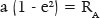
Let be RA the radius of curvature at this point (A) of the surface. By the formula of refraction on a spherical surface, the relationship between the image’s position, relative to A (i.e., q) and the radius of curvature (RA) can be established according to the respective refractive indices (ni an nr) as

which can be rewritten according to the focal power assigned to surface (F):

Hence,

The spherical non-aberration condition of this surface presupposes that any point P of that surface has the image of the object(located at the infinite distance) formed exactly over Q, i.e., coinciding with it. The direction of the incidence of radiation on P is therefore parallel to the direction of incidence on point A. By the normal line to point P and (still) regardless of the surface’s shape, the geometric relationships of this coincidence can be established (Figure 11).
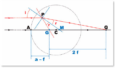
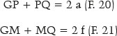
Hypothesizing that G and Q are the foci of an ellipse to which P belongs, the following relationships will apply to triangles GPM and MPQ, respectively:
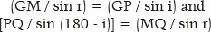
Hence,
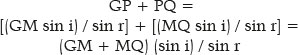
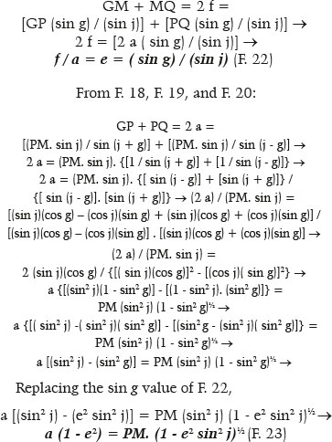
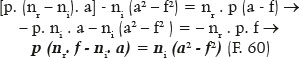
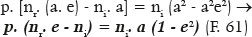
Since in ellipses, GP + PQ = 2 a, i.e., the sum of the distances from the considered point (P) to each focus (G and Q) equals the length of the ellipse’s major axis; and GM+ MQ = 2 f. Thus,

Since (f/ a) = e measures the ellipse’s eccentricity, the fundamental relationship is established between its “shape” (described by its eccentricity, e) and the relationship between the refractive indices of the media considered, such that the incidence of parallel rays on any points on this surface (i.e., all) produce refracted rays that converge to a single point (Q), one of the ellipse’s foci:
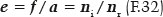
In other words, for a curve to not exhibit spherical aberration, it must be elliptical and of an eccentricity that corresponds to the ratio of the refractive indices of the incidence and refractive media separated by it.
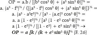
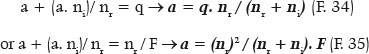
Once this condition is satisfied, infinite surfaces may exist, each with the specific focal length (AQ = q) that is a function of the radius of curvature of the apical point of the major axis (A), i.e., RA, whose value has already been defined (F. 30 and F. 31). Thus, in figure 11, as AG = a − f, the generically formulated focal length is the following:

Finally, the variables of the ellipse can be determined from q (image focal length ) or F (surface’s focal power), conventionally taken with respect to the curvature radius of the apical point of the ellipse’s major axis (RA). Hence, for the length of the ellipse’s semimajor axis (a),
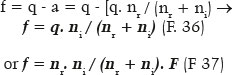
For the semifocal axis length (f),
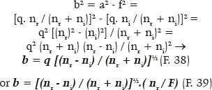
For the semiminor axis (b),
Other relationships between these variables can also be obtained (for example, a - f or a / b, etc.). Table 3 summarizes those formulations for surfaces without spherical aberration.
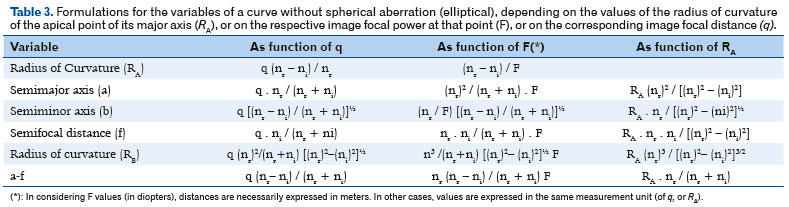
Some relationships are purely dependent on the ellipse itself, such as the eccentricity (e) that defines it, or others that can be deduced from the formulas already presented:
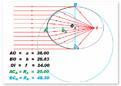
As a numerical example, consider a surface separating two media, with refractive indices of 1.0 for incidence (ni = 1.0) and 1.5 for refraction (nr = 1.5). To determine the eccentricity of the (elliptic) curve such that it does not produce spherical aberration, e = ni/nr = 1.0/1.5 = 0.666... Be the radius of curvature at the apical point of its major axis equals to 20 cm (RA = 20 cm). The focal power of this surface (object located at an infinite distance from the surface) is F = (1.5 − 1.0) /0.2 m = 2.5 D. The image focal length of this surface is q = 1.5/ F = 1.5/2.5 = 0.6 m = 60 cm. In this curve, the semimajor axis (a) is then (calculation that can be done, alternatively, either from q = 60 cm, or from RA = 20 cm, or from F = 2.5 D), a = 36 cm (or 0.36 m, if the calculation is done by the formula containing the F-value). The semifical axis is f = 24 cm. The semiminor axis is b = 720½ ≈ 26.833 cm and the radius of curvature of the apical point of the minor axis is RB ≈ 48.299 cm. By Snell’s law, assuming an incident radius parallel to the optical axis and tangentiating this apical point of the minor axis (a purely mathematical conjecture), we have

for f = 24 cm and a = 36 cm, expressing the eccentricity ratio of this curve. Obviously (a − f) = 12 cm, whose calculation can be confirmed by any formulas presented for the variable (a - f) in table 3.
Table 4 summarizes values of the variables of curves without spherical aberration, according to the refractive index nr, in case the medium of incidence is air (ni = 1.0).The calculations for the above mentioned example (q = 60 cm and Figure 12) correspond to those in the third row of table 4 (nr = 1.500).
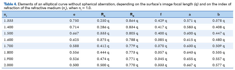
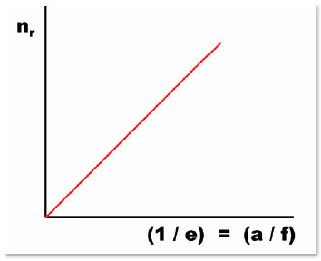
A very important relationship is the eccentricity of the curve, such that it does not show spherical aberration when the incidence medium is air. In this case, ni = 1.0 and the expression of eccentricity is expressed by the inverse of the index of refraction of the refractive medium (nr), that is, e = 1/nr. Reciprocally, e-1 = nr = a / f. This is an interesting simplification for it shows the perfect linearity between the index of refraction nr and the relationship between the lengths of the major axis (2 a) and the interfocal distance (2 f) of the surface without spherical aberration (Figure 13).
Positioning the center of curvature
Figure 14 shows the procedures that graphically determine the position of the center of curvature of any point on an elliptical surface:
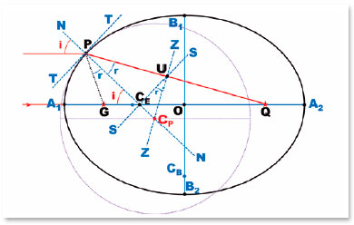
1) Draw the tangent line (TT) to the point of the surface (P) which center of curvature is to be determined.
2) Draw the normal line NN perpendicular to the surface tangent (TT) at the point considered (P). NN will contain the center of curvature of the surface at that point (P).
3) At the crossing point of the normal line (NN) with the major axis of the ellipse (A1A2), a point (M) is defined. By M, is drawn a line parallel to the tangent (TT), i.e., the SS line.
4) From the crossover point of the SS line with the line that joins point (P) to the farthest focus (Q), line PQ, i.e., point U, is drawn a perpendicular to the PQ direction (considered to be the refracted ray), line ZZ.
5) At the intersection of line ZZ with the normal line to point P (line NN), the center of the osculating circle to point P (point CP) is located. PCP = RP is the radius of curvature of that circle.
Figure 15 is the reproduction of figure 14, purged from the elements used to determine point CP. It makes it easy to understand the following geometric deduction.
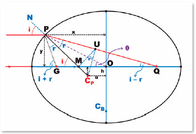
The coordinates of the point P and CP are P (x, y) and CP (u, h) , respectively. Hence, the radius of curvature (RP) is determined as

The relationships between the functions of the elliptical curve (a, b, f, RA), the coordinates of one of its points (x, y, θ) and the respective functions related to refraction (i, r, ni, nr, q, F, etc.) the following formulations are obtained:
From the PGM triangle, by the law of sines,

From the MPQ triangle, by the law of sines,

Yet,
Hence,

Finally, since GM + MQ = 2 f,
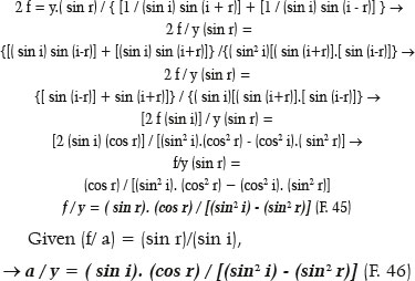
Alternatively, the equation can be converted to the calculation of i (or r) according to y and a (or f, or θ, etc.). Thus, from F. 45,
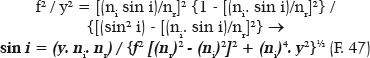
E.g., for nr = 1.5, ni = 1.0, f = 24 cm, and for y for θ = 40° (by F. , being a = 36 cm and b = 720½ cm, it comes y = 20.06115396 cm), results sin i = 1.5 y / (900 + y2)½, and thus, i = 56.49204167°. (Note that this result can also be obtained from F. 24, when j = i.)
The value of the “apparent” radius of curvature (PM = RM, Figure 15 and F. 44) can then be calculated as PM = RM = 20.06115396 / sin 56.49204167° = 24.05964716 cm (result also identical to that obtained by F. 25). The true radius of curvature (PCP = RP) is easily calculated from the PUCP and PMU triangles, respectively:

from which RP = 34.81831666 cm.
Hence, the values of the coordinates of the center of curvature (u and h) can be derived as follows:
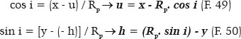
Table 5 shows approximate values (up to the third decimal place) of the values of the coordinates of a point P (x, y) depending on the angle (θ), those of the line (OP) between that point (P) and the center of the ellipse (O), the coordinates of the center of curvature (u and h), the “apparent” radius of curvature value (PM = RM) and the true (RP) value as well as the angle of incidence (i) and that of refraction (r) corresponding to the points which coordinates are considered.
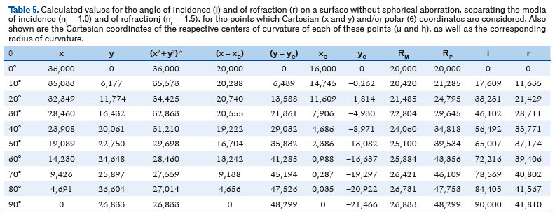
Table 6 complements table 5, showing (in the penultimate column) values of the coordinate (m,0) of point M, i.e. the “pseudo” center of curvature of point P, that is, the place where the normal at that point crosses the major axis of the curve (its main optical axis), given by the equation

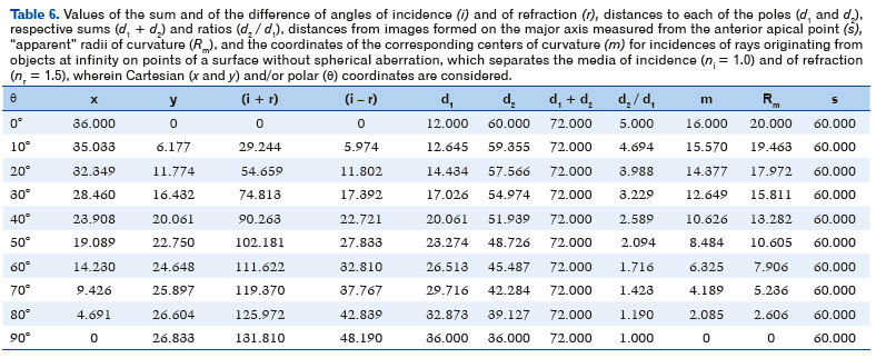
or of its respective distance to the anterior apical point (that is, the distance A1M = Rm, Figure 14). Note that Rm corresponds to the value of the true radius of curvature, when i = 0° (Rm = RA) and the value Rm = PM cos i, when 90° > i > 0°. In fact, for these cases, m + Rm = x.
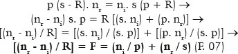
It also shows some variables supporting other possible calculations, as well as their relationships. In fact, in certain cases, it may be interesting to know the value of the distance from each focus to the point P (where incidence and refraction occurs), that is, GP = d1 and QP = d2 (Figures 14 and 15), as well as the result of its sum (always equal to the ellipse’s major axis, i.e., d1 + d2 = 2 a = 72.000 cm, in the example considered) and of its ratio (d2/d1), incidentally, equal to the ratio between the sine of the sum and of the difference between the angles of incidence (i) and of refraction (r) They may be deduced from figure 15:
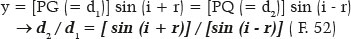
Finally, it considers the s value, which as expected, must correspond to distance A1Q (Figure 14), that of the surface’s image focal length :

E.g.: for θ = 40°, the corresponding values are (Table 6 ): x = 23.908 cm, y = 20.061 cm, (i - r) = 22.721°, from which we obtain s = 60.000 cm.
The eccentricity of the curve of no spherical aberration as a contingency of the object position
The fact that the eccentricity of an elliptical curve justifies the absence of spherical aberration in the refraction of the image formed by it from incident rays parallel to the optical axis does not mean that this property applies to other incidences, i.e., to other positions of the object in relation to that surface. In fact, if an object located at an infinite distance forms an image 60 cm from the surface, as exemplified, this corresponds to an anterior apical curvature radius of the surface (RA) equal to 20 cm, which conditions all geometric variables of the curve (a = 36 cm, f = 24 cm, b = 720½ cm, whose relationships are typified by the eccentricity e = 0.666..., as demonstrated for media with refractive indices ni = 1.0 and nr = 1.5). Meanwhile, an object at any other distance from this apical point will necessarily form its image subject to the laws of refraction, at different distances, as per the expressions F. 06 or F. 07.

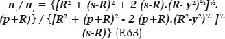
Thus, under the pre-established conditions for the surface without spherical aberration of apical curvature radius RA = 20 cm, nr = 1.5, and ni = 1.0, we get p = 120 cm, q = 90 cm. On the same elliptical surface previously used as an example, the incidence of another incident rays of this object to other points of it (such as P, Figure 16) leads to algebraic relationships, which allow the calculation of the distance s at which the image is formed.
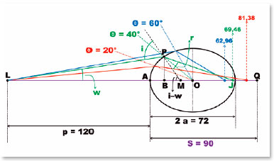
For the LBP triangle, being LA = p, AB = (AO - BO) = (a - x), PB = y (taken from the θ = 40° value), angle w is determined:

from which one obtains w = 8.636 cm. To determine the direction of the refracted ray (angle r), the value of the angle of incidence (i) is required. The latter can be determined from the inclination of the apparent radius of curvature (PM = RM) or of the true (RP) relative to the ellipse’s major axis, i.e., i − w. The apparent radius of curvature of point P is known (PM = RM). Hence,

therefore (i − w) = 56.492°, hence i = 65.128° which, by rhe Snell’s law gives r = 37.217°. BQ is calculated next, as follows:

This results tan 19.275° = 20.061/BJ; thus, BJ = 57.365 cm. Finally, for the desired unknown value, s = AJ = AB + BJ:

that is, s = 12.092 + 57.365 = 69.457 cm. For other y-values (corresponding to other supposedly known values of the coordinate θ), the calculations are analogous, leading to the values shown in figure 16.
In short, the curve whose shape (eccentricity) is suitable for nullifying the spherical aberration of images of an object located at infinite distance is unable to do so if the object is at a finite distance. For a closer object, a curve with a greater eccentricity would be required. In other words, “asphericity” (condition of no spherical aberration) ( which can be defined by the eccentricity value of the curve) is not applicable for any distance. Moreover, spherical aberration is not caused by a presumed spherical surface, but rather it is a property inherent to the very nature of refraction.
Therefore, despite occurring on spherical surfaces, the term “spherical aberration” is absolutely inappropriate since it also occurs on elliptical surfaces, even those which can be defined as “aspherical” for objects at infinite distances, but do not keep such a property for images of closer objects. A more convenient label for such a type of refractive deffect might be of surface (or diopter) aberration or of aberration of surface (diopter) curvature. Curvature aberration can simply lead to confusion with “field curvature,” which are aberrations of other phenomena.
Calculation of the eccentricities that maintain asphericity at finite distances
The relationship between the cancelation of “surface” (diopter) aberration (“spherical” aberration), caused by (1) a certain eccentricity of the curve (elliptical, as has been studied)—in turn dependent on the refractive indices of the medium separated by the surface—and (2) the object’s distance, which images must form on a single point (image “focus” ), regardless of the incidence on the surface, can be sought. In fact, it is possible to assume that “asphericity” could be also obtained for images of objects located at finite distances with curves of greater eccentricities. For an object at a given distance (for example, p = 120 cm), located on the optical axis of any curve that separates medium with refractive indices ni = 1.0 and nr = 1.5 and has a radius of curvature RA = 20 cm at its apical point (coincident with the optical axis), i.e., with a focal power (nr - ni)/RA = 2.5 D, and considering a null incidence (i = 0°) it will form the respective image, also on the optical axis, always, at the same distance (s = 9 ). In any case, although infinites of these curves are possible, only one elliptic will also have the sum a + f = 9, thus extracting a specific value for its eccentricity, which can then be calculated.
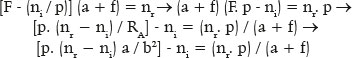
If L is the considered light source and if Q is the point upon which the image of the refraction produced by the null incidence is formed, Q will be one of the foci of the elliptical curve. Thus, the distance from this source (L) to the anterior “pole” (vertex) of the ellipse (A), LA = p, is the distance from the object to the surface; and AQ = a + f is the distance at which the respective image is formed. (Points L and Q are supposed to be coaxial to the ellipse’s major axis, or optical axis of the surface.) By the law of refraction,the paraxial ray equation:

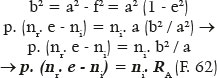
Variables RA (radius of curvature of the anterior apical point of the ellipse), a (its major semiaxis) and f (its semifocal distance ) are thus automatically related to the variables related to refraction, ni (index of refraction of the incidence medium), nr ( index of refraction of the refractive medium), p (distance from the object to surface), or F (focal power of the surface). The distance from the image to the anterior pole of the surface (s) is automatically determined (s = a + f). In fact, this equation (F. 59) can be rearranged:
But given , b2 = a2 - f 2
More concisely,
Further, depending on RA, since
In fact, for objects at infinity (p = ∞), nr. e = ni, as already demonstrated. Thus, for the object at infinity (p = ∞) the eccentricity of the “aspherical” curve (e) equals the reciprocal of the refractive indices of refraction on the incidence (ni) and refractive (nr) media. For distance p = 120 cm, RA = 20 cm, ni = 1.0, and nr = 1.5, the eccentricity of the curve is
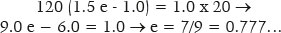
which is greater than the eccentricity of the spherical curve for the object at infinity (e = 1/1.5 = 2/3 = 0.666...). This eccentricity (e = 2/3) is therefore not appropriate to nullify the spherical aberration for images of an object situated at other distance.
The value of this ellipse semimajor axis (a) is determined by:
i.e., a = 20/[1 − (0.777)2 ] = 50.625 cm; hence f = 39.375 cm and b ≈ 31.820 cm.
However, for other incidences on this surface, considering the distance of 120 cm (= p) from the object to the front vertex of the major axis of such an elliptical surface, spherical aberration still persists, as table 7 shows (second column). Finally, to possibly nullify the “spherical” aberration (or curvature aberration) corresponding to an object at a finite distance, this curve with that “typical” eccentricity (e = 7/9) shows nothing special compared to others (e.g., with e = 2/3, as seen in Figure 16). It only represents the maximum eccentricity value, such that a + f = 90 cm and RA = 20 cm. In fact, for an ellipse of greater eccentricity, such as e = 0.8, with a = 50 cm and f = 40 cm, then RA = b2/a = (a2 - f2)/a = 18 cm.
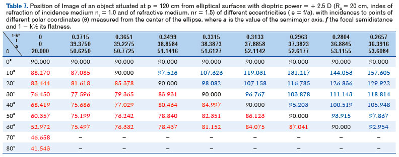
For this ellipses family (with a + f = 90 cm and RA = 20 cm) other eccentricities may be specific to values of other incidences, as table 7 shows. Remember that for a finite distance and a non-axial incidence, the applicable formula for the calculation where the distance at which the image (s) is formed equals a + f = a + ae = a ( 1 - e) is F.5:
in which the value of the radius of curvature (R) varies according to the point of incidence but with a specific value (corresponding to y), such that the image forms at distance s = 90 cm.
The results in table 7 are paradigmatic:
a) The second column corresponds to a circular curve (zero eccentricity, flatness 0). Note that the more peripheral the incidence point (the greater the angle θ value), the closer to the surface the corresponding image forms (red numbers), which means the so-called positive “spherical” aberration.
b) Curves of greater eccentricity (and greater flatness) will progressively correct this aberration. E.g.: for eccentricity e = 37.8858/ 52.1142 (seventh column from the left) the aberration is corrected to the incidence of 40° (the image forms at exactly 90.000 cm, as desired). For this inclination (40°), greater eccentricities will produce positive aberrations (red colored numbers) and smaller eccentricities will produce negative aberrations (blue colored numbers). (Exception made to the circle, second column, where e = 0/20.0 = 0.)
c) Elliptical curves can’t prevent the “spherical aberration” of images of objects located at a finite distance. At best, a curve with a certain eccentricity promotes the coincidence of the position of the image produced by null incidence (in this case, 90 cm from the surface) only for another incidence. The table shows the eccentricities of the curves corresponding to incidences of 10° to 70°, although curves of intermediate flatness between those shown are also possible. E.g.: between the 0.3651 flatness curve (which matches the 10° incidence ) and the 0.3499 (which matches the 20° incidence ), an intermediate flatness curve will promote the formed image at 90 cm from the surface for a certain specific incidence, between 10° and 20°.
d) The curve of a given eccentricity produces negative aberrations for incidences lower than that which promotes the desired position of the image (at 90 cm); and positive aberrations for incidences greater than the specific.
e) Thus, a curve promoting total asphericity (images positions always at 90 cm) should have a decreasing eccentricity (and/or flatness ); in this case, starting from e = 7/9, third column, with an increasing angle of incidence. It would not be an elliptical curve, therefore.
f) Even if such a curve could then be constructed, it would serve to neutralize the aberration of “sphericity” for, only and specifically, the position of the object at p = 120 cm (and mediums of incidence and refraction such as those aforementioned). For other distances and other indices of refraction , a new curve specific to each case should be constructed.
In fact, the fundamental equation by which one can understand the relationship between the geometric properties of an elliptical curve and the basic law of refraction (by Snell and Descartes) is that of F. 22, that is, e = (sin g) / (sin j), where j = i - w (for finite-distance objects) and g = r, the angle of refraction obtained from this incidence. In other words, the equivalence between the angle of incidence (i) and that of refraction (r) - which must always obey Snell’s law- is also subordinated to the ellipse’s geometry with its specific (e) eccentricity. Despite not explicit in table 7, this F. 22 is only satisfied at a specific angle (i - w), corresponding to an incidence (i) which relation to the angle of refraction (r) expresses the eccentricity of the curve (e) value. Tables 8 and 9 show values of some of the variables of the ellipse geometry for different angles of incidence (i) relative to the ellipse’s center (θ), when w values also vary, for ellipses with eccentricities e = (f / a) = 38.8584 / 51.1416 = 0.7598 (Table 8) and e = 37.8858 / 52.1142 = 0.7270 (Table 9). Note the highlighted (red) values of s = 90.0000 (the position of the image satisfied, in each case, by refraction for angles θ = 20° in Table 8; and angles θ = 40° in Table 9) and those of the respective relations of the sines of the angles (i − w) and r, coinciding with the value of the corresponding eccentricity of the curve (e = 0.7598 in Table 8; 0.7270 in Table 9), respectively. In other cases, this coincidence is inexistent and the image position does not occur at the desired point (s = 90.0000 cm).
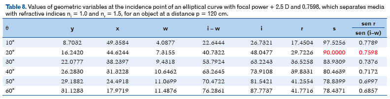
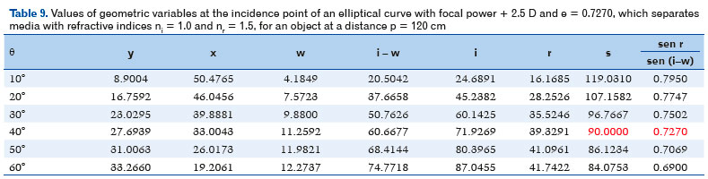
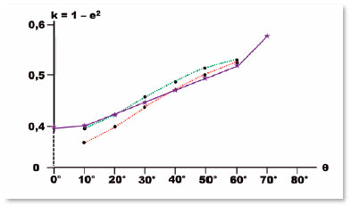
Figure 17 also shows the relationship between an ellipse’s variable k = 1 - e2 and the polar (angular) coordinate of a point (measured from its center), which refracted ray therein (from an incident ray originating from a finite-distance object) reaches the optical axis in the same place where this object’s image corresponding to zero incidence is formed. Note that this ellipse variable in which this situation occurs is greater the more peripheral the point where the refraction is considered (purple line), i.e., for each angle taken from the center of the ellipse, an increasing variation of k (as a function of the angulation value) would be adequate to satisfy such conception. Contrarily, for this desired asphericity to occur for any point on the curve, the representation of a single k value would be that of a straight horizontal line (perpendicular to the ordinate axis and parallel to the abscissas axis).
The different positions of the curvature centers of each point of the surface and their refractometric consequences
One of the peculiarities of the elliptical curve is that there is a specific center of curvature for each of its points. Its derivation was outlined in figure 14. The calculation of its coordinates, as well as the value of the actual curvature radius (RP = PCP) and “apparent” (RM = PM) curvature radius were explained by figure 15 and by F.49 and F. 50 (for coordinate values), F. 27 and F. 43 (curvature radius RP values by polar and Cartesian coordinates, respectively), F. 44 (apparent radius of curvature values PM = RM) and F. 48 (values of the relationship between RP and RM).
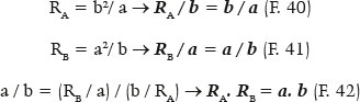
The geometric location of the various centers of curvature, from the anterior apical point (A), RA (F. 28) to the vertex of the minor semiaxis (B), RB (F. 29) and their relationships (F. 40-42), crossing the intermediate curvature centers, is the so called ellipse’s evolute (Figure 18).
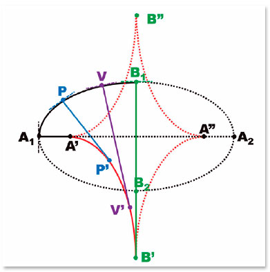
In ellipses, the points of greatest curvature (A1 and A2, radii of curvature A1A’ and A2A,” Figure 18), have the centers of the respective osculating circles (i.e., the centers of curvature of these points) within the ellipse, whereas the points of smallest curvature (B1 and B2,, curvature radii B1B’ and B2B,” Figure 18) have the centers of the respective osculating circles (i.e., the centers of curvature of these points) either outside or inside the ellipse (see Figure 12). The ellipse’s evolute is analytically described by equation:

The radius of curvature (RP) value of any point of an ellipse can be determined by both F. 27 and F. 48. It always requires the knowledge of two of the ellipse’s variables (a, b, f, or e, through which the other two are calculated) as well as defining the point for which the respective radius of curvature is required. This raises the need to know two of their coordinates (the Cartesian, x and y, or one of them plus the angular coordinate θ). For example, by replacing the value of
In fact, if j = 0°, RP = RA = a (1 - e2) = a. (b2/a2) = b2 / a, ratifying the F.28. If j = 90°, from F. 65 it comes RP = RB = a (1 - e2) / (1 - e2)3/2 = a / (1 - e2)½ = a / (b2/a2)½ = a / (b/a) = a2/b, ratifying the F. 29.
From F. 48 and F. 44, the angles i and r may be replaced by their respective generic versions, j and g, where (sin g)/(sin j) = e, hence: y = RM. sin i = (RP. cos2 r). sin i = RP (1 - sin2 r). (sin i) = RP (1 - sin2 g).( sin j)→
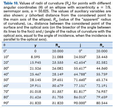
Thus, for example, for the ellipse with a = 50.625, e = 7/9 and θ = 10°, from F. 16 it comes y = 8.594755891 . Hence, by F. 25, RM = 21.08759556, and thus, j = arc sin (y / RM) = 24.05252876°. Finally, either by F. 65, F. 66, or F. 67, we can determine RP to be 23.44343249.
Table 10 shows the radius of curvature (RP) values for points of this ellipse, with different angular coordinates relative to its center (θ), as well as those of other corresponding variables. Figure 19 depicts the variation of these curvature radii and the corresponding dioptric values (for a curve separating media with indices of refraction ni = 1.0 and nr = 1.5).
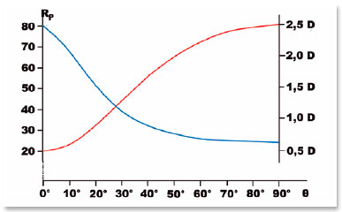
It is easy to understand from figure 19 that the dioptric values of this aspherical elliptic curve progressively reduces as the incidence (parallel to the optical axis) becomes more peripheral (blue line). It should be noted, however, that a prolate curve is being considered, i.e., with the major axis coincident with the horizontal plane. If the elliptical curve is rotated 90° around an axis perpendicular to the plane of its representation, passing through its center, its radii of curvature and respective centers do not change relative to the ellipse. Instead, it assumes an oblate shape, i.e., with the minor axis coinciding with the horizontal (Figure 20) and therefore with decreasing radii of curvature and respective increasing dioptric values as more peripheral incidences occur.

The multifocality of elliptical curves
As the dioptric values of a lens at its different points are directly proportional to those of its respective curvatures, i.e., the greater the curvature of a surface at a given point (smaller the radius of curvature therein), the greater its respective dioptric power, the elliptical curves naturally lend themselves to satisfy multifocality, according to the incidence and/or the direction of the refracted ray; in other words, according to the direction of the visual axis that crosses it.
In fact, by choosing a dioptric value (i.e., a curvature) for a given point on a surface, it is possible to set a new curvature (greater or lesser) for another point, such that it features a transition of the corresponding dioptric values (progressive or regressive) between them. More common is to want a certain dioptric value for a “far” distance (e.g., +1 D) and a higher one for a “near” distance (e.g. + 4 D), which usually occurs at downward gaze positions. In a myopic person, the case would be a variation from -5 D to -2 D, for example, but regressive variations (or semiprogressive, different names to basically express the same concept) may also be convenient. Although it is not this dissertation’s aim to discuss the convenience and applications of such clinical concepts, nor the technical difficulties of operating their fabrications, the principles that govern this multifocality (much desired in ophthalmological practice) will only be addressed briefly.
Consider an elliptic curve which represents the first (or anterior) principal plane of a lens, i.e., the imaginary place where all the refraction of incident (and refracted) rays takes place, whose effect would be of a decreasing multifocal dioptric power in a prolate curve (Figure 18), or crescent in an oblate (Figure 20). Due to the greater applicability of increasing multifocalities, the example will be restricted to this concept and shape (oblate) of the ellipse, whose explanation will be developed based on figure 21.
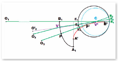
Let be R1 the retinal (foveal) image of the object O1 (located at infinite distance) formed by the “lens” (the abstract surface A1B1). The dioptric power of this surface at point B1 is assumed to correct a possible optical error of the ocular system, so that its value can be empirically determined. Note that the visual axis (line R1C E1 O1) is coincident to the radius of curvature (B1B’) at point B1, i.e., is tangent to the curve’s evolute at B’. Another line tangent to the ellipse’s evolute at P’ may be made coincident to a new position. of the visual axis to fixate object O3 (line R3CE3O3), so that PP’ is the radius of curvature of the surface at point P’, i.e., the point where the visual axis to fixate the object O3 (line R3CE3O3) cross the surface. The optical power of P may be chosen to allow the required optical correction for objects (O3) at “near distances” (the so-called “addition” over the required optical correction for “far distances”). Therefore, if the surface’s dioptric power values for points B1 (“far distances”) and P (“near distances”) are chosen, that means, if radii of curvatures of surface’s points B1 and P are known (as function of variables nr and ni), the curve between B1 and P is also determined.
Intermediate surface’s points between B1 (the longer radius of curvature, therefore the lesser dioptric power) and P (the shorter radius of curvature, therefore the greater dioptric power) will have intermediate radius of curvature and, therefore, intermediate dioptric powers, so that a surface’s “multifocal” effect results. Note, however, that as B’ and P’ are tangents to the curve’s evolute and coincident to the optical axis, the tangent point to the evolute at any other intermediate point (as V’, which corresponds to the surface’s point V), lies below the center of rotation C (for which passes the visual axis). Therefore, the visual axis (R2CE2V) and the surface’s radius of curvature at V (= VV’) although having a common point of coincidence (V) are not collinear. The angle between them (R2VV’) is equal to the angle of refraction (r) at V, so that there exists at this same point (V) an angle between the directions of the actual position of the object in space (O2), line VO2 and its perceived one (O’2), line VO’2, the angle of incidence (i).
Although the rationale of the multifocality of an elliptical curve is so relatively simple, the calculations are complex and will not be here presented.
Appendix: sphere, spheroids, and ellipsoids
Refractions occur on surfaces, or on entities of three-dimensional space that can be analytically described by specific values in each of its axes. Circles, ellipses, and other curves are “figures,” or flat sections (in two-dimensional space) of realities (in three-dimensional space). In other words, they are merely pictorial representations (lines) of solids which surfaces (three-dimensional) separate the media in which refractions occur. Thus, it is appropriate to extend the study on the “realities” of which these figurations now addressed (elliptical curves) are mere simplified (planar) representations
In ophthalmology, it is customary for the three spatial axes to be named as “z” (vertical), “y” (horizontal, longitudinal, i.e., coincident with the visual axis) and “x,” also horizontal, but perpendicular to the “y” axis, separating “left” and “right,” or “lateral” (or “temporal”) and “medial” (or “nasal”), mutually orthogonal, i.e., each axis belonging to two planes and perpendicular to the remainder. Thus, although the structures may have any sizes, they can be represented by their proportional dimensions on each of these axes.
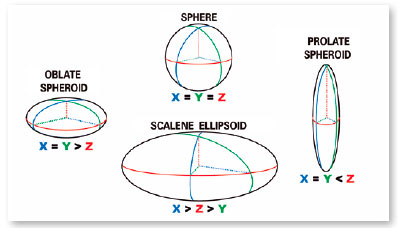
A volume represented by three axes of equal dimensions (x = y = z) is a sphere. If two of them are equal but different from the third, the possibilities are six (x = y > z; x = y < z; x = z > y ; x = z < y; y = z > x; y = z < x) and the represented volumes are spheroids (Figure 22). In fact, they are solids generated by the rotation of an ellipse, around one of its axes (Figure 23) and, therefore, the sections perpendicular to that axis of revolution will always be represented by circles (hence the name “spheroids”). Finally, when the three axes are described by different values, the possibilities are six more (x > y > z; x > z > y; y > x > z; y > z > x; z > x > y; z > y > x) and solids called scalene ellipsoids. (Figure 24, showing one of them).
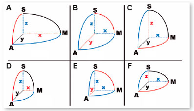
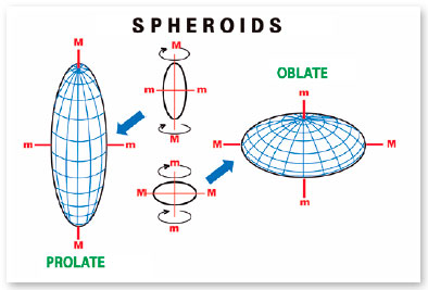
Note that in the prolate form (similar to a kibbeh, a rugby ball, or a football) one of the axes is longer than the two others (equal) and in the oblate form (similar to a dragee, or a thickened disc at its center, like a “flying saucer”), one of the axes is shorter than the other two (equal). However, always considering the relative position of the axes as coincident to that of the eye (y, the longitudinal, or anteroposterior; z, the vertical, or super-inferior; and x, the transverse, or latero-medial), the differences between these presentations appear. For example, in prolates by the disposition of the major axis (their “acute peaks” ) and in oblates by the disposition of the minor axis (their “ flat poles”).
Thus, when the longer axis is y (longitudinal), the vertical (between A and S) and horizontal (between A and M) curves will be elliptical and equal to each other (Figure 22b) and regardless of the surface appearance (like, for example, the cornea) is “conical”, there is no astigmatism (difference in dioptric powers between them). Thus, also, if the minor axis is the y (longitudinal), the vertical curve (between A and S) and the horizontal (between A and M) will be elliptical and equal to each other (Figure 22 e); the surface appears “conical” in these two planes (or meridians) but also without astigmatism. When the major or minor axis is x, the transverse (respectively, Figures 22 a and 22 d), there is a difference between the curve of the horizontal plane (between A and M, elliptical) and the vertical (between A and S, circular), therefore causing astigmatism. In figure 22 a, the plane (or meridian) of lesser curvature ( greater curvature radius, lesser dioptric power) is horizontal, configuring an astigmatism “with-the-rule”; in figure 22d, the greater curvature (smaller curvature radius, greater dioptric power) is horizontal, representing an example of “against-the-rule” astigmatism. Thus, also, when the major or minor axis is the vertical (z, respectively figures 22 c and 22 f) there is a difference between the curve in the vertical plane (between A and S, elliptical) and the horizontal (between A and M, circular), so that figure 22 c represents an “against-the-rule” astigmatism and figure 22 f represents an astigmatism “with-the-rule”. Although it cannot be guaranteed (since in the composition of ametropias the axial factor is relevant), it is at least allowed to conjecture that errors related to curvatures induce refractometric errors; therefore, astigmatism: myopics in their excesses (in oblate spheroids, Figures 22, d, f), or hyperopics in their insufficiencies (in the prolate spheroids , Figures a, c). Remember that, in these astigmatisms, the pointed prolate form, the longer axis is vertical (Figure 22 c) or transverse (Figure 22 a); and in the oblate, or flat form, too (Figures 22 d and 22 f, respectively), as opposed to the condition in which the z and x axes appear equal (Figures 22 b and 22 e), which raises apparently paradoxical interpretations regarding the respective curvatures considered.
SYNOPSIS
Introduction: Knowledge about refraction is shown to be essential in ophthalmic practice. Refraction is a physical phenomenon dependent on the change in the speed of propagation of radiant energy in its transition from a medium from where it originates (the medium of incidence) to another, by which it follows (the medium of refraction), governed by a law of great simplicity, which dictates the relation of such speeds (or, equivalently, relative numbers that represent them, the specific refractive indices of each of these media), and the directions in which the radiant energy wavefronts propagate. The measurement of these directions is specific to each point of the surface of separation between the media of incidence and of refraction and depends on an imaginary line perpendicular to that point (its normal). Although refraction is a punctual phenomenon, only considering the relation of directions of the incident and refracted radiant energy, it is, in broader terms, dependent on the surface to which such a point belongs.
Curvature of a surface: The characterization of a point on a surface is determined by its curvature, a concept that is quantified by the length of a straight line, the radius of curvature of the point in question. In geometric optics, although the direction in which the image of an object is formed depends only on Snell’s law, its position is subjected to the radius of curvature of the point where the refraction takes place. The radius of curvature is infinite on flat surfaces, finite and constant in spheres (or circles), finite and variable in other curves (such as conical sections). All corrective lenses for ocular optical defects are formed by curved surfaces (at least one). Ocular refractometry texts address refraction on flat (prisms) and spherical (lens) surfaces and are limited to them. Refraction on spherical surfaces is inherently defective (spherical aberrations). Spherical aberration-free (aspherical) and multifocal lenses require the development of optics based on varying radii of curvature at different points on the refracting surface.
Refraction on spherical surfaces: The principles and formulations of this type of refraction are reviewed for the generic case of the position of the image of an object point located at a finite distance. Based on these principles, the paraxial ray equation, that of when the object is located at an infinite distance, and that of the basic formulation of the surface dioptric power are derived. Despite the relative simplicity of its study, refraction on spherical surfaces has as an intrinsic consequence: spherical aberration. This corresponds to the distribution of incident radiant energy, for example, in a beam of parallel rays (flat wave fronts) over an extensive region of space where the various crossings of the various refracted rays occur, delimited by a surface (the caustic).
Aspherical Surfaces: The ones concentrating in a single point (the image focal point, when the incidence comes from infinity) all the refracted radiant energy. Their design requires that the farther from the optical axis the incidence is, the smaller the radius of curvature of the surface becomes, when compared to that of the surface’s vertex (located on its optical axis). This notion corresponds to what occurs in ellipses (and other curves), which shapes can accentuate the spherical aberration of spherical surfaces (aberrations called “positive”), reduce it and even neutralize it (by an aspherical elliptical surface) or invert it (producing “negative” spherical aberrations).
The semantic question of asphericity: The different ways in which ellipses and their varied results can be presented, raises the discussion about the inappropriateness of the term “spherical” aberration, as it does not depend exclusively on spherical surfaces and may occur in elliptical surfaces (in a “positive” or “negative” way). It is proposed to use the terms of superaberrant surfaces for those which produce “positive” aberration, greater than that of the spherical aberrations of a sphere, subaberrant surfaces when they stil produce “positive” aberrations, but lesser than that of spherical surfaces), inaberrant when aberration is eliminated (the aspherical surfaces themselves) and contraberrant if they produce negative aberrations. With this terminology, any oblate surface will be superaberrant, whereas among the prolates, sub-aberrations (“positive”), inaberrations, or contraberrations (“negative”) may be found.
The geometry of ellipses: The geometric properties of the ellipses, their terms and relationships are succinctly presented.
Refraction on a surface without spherical aberration: Based on the geometric properties of the ellipses, the condition under which the refraction of an incident ray parallel to the optical axis on one (any) of its points gives a refracted ray that meets the optical axis at one of the foci (the focal point surface image) is examined. It is possible to formulate that, in these cases (incidence of planar wavefronts), asphericity is achieved when the eccentricity of the ellipse (e) equals the ratio of the indices of refraction of the incidence (ni) and refraction (nr) media, i.e., e = ni/nr. Equations showing the relationships between the different surface properties and the values of its dioptric power are developed as well as the eccentricity values so that the surface be inaberrant (aspherical) according to the index of refraction of the medium of refraction, when that of incidence is air (ni = 1.0).
Positioning the center of curvature: We present the method by which the position of the center of curvature of any point of an ellipse can be determined graphically, as well as the analytical method for knowing its coordinates, the value of the respective radius of curvature and other relationships between the properties of these “aspherical” ellipses.
The eccentricity of the spherical non-aberration curve as a contingency of the object’s position: It is shown that the curve for which “asphericity” is obtained for the incidence of planar wave fronts (objects situated at infinity, rays parallel to the optical axis) does not maintain this quality for objects at finite distances, i.e., the eccentricity of the asphericity promoting curve is a function of the distance from the radiation source.
On the calculation of the eccentricity that maintains asphericity at finite distances: The fact that the shape (eccentricity) of the curve that provides asphericity for the formation of the (unique) image of an object located at infinite distance does not maintain this quality to the object’s position at other distances, does not mean that a relationship cannot be found between a specific eccentricity and the distance from the source. This possibility is studied, and we find that there is in fact an appropriate eccentricity such that for a specific incidence, the position of the image of an object located at the finite distance coincides with that obtained from the definition of the focal power of the surface (i.e., with that of the null incidence). However, for smaller and larger angles of incidence on the curve that ensures this “pairing”, the aberrations remain negative and positive, respectively. Likewise, for a certain incidence, curves with smaller eccentricities produce negative aberrations and those with larger eccentricities will produce positive aberrations. The variability of eccentricity necessary to produce the coincidence of images of an object located at finite distance, depending on the angle of incidence, means that an elliptical curve (single eccentricity) cannot satisfy that condition (asphericity for images of objects situated at finite distances). objects).
The different positions of the curvature centers of each surface point and their refractometric consequences: The study of the positions of the centers of curvature of the different points of an elliptic curve is resumed to describe their proper “geometric place” , a new curve, the ellipse’s evolute and what occurs when this ellipse is rotated around an axis perpendicular to its figure, making it pass from one “form” (prolate) to another (oblate). Although the eccentricity (descriptive of the “formal” relationships of the ellipse) remains the same, its spatial arrangement (with the longest axis horizontally or vertically) will transform decreasing variations of curvatures (increasing their respective radii, into curves called prolates) into increasing ones (oblates curves).
The multifocality of elliptical curves: The variability of the values of the curvature radii of an elliptical surface (defined by its eccentricity) is a matrix of what refractometry calls “multifocality.” Thus, increasing (“progressive”) or decreasing (“regressive”) dioptric power lenses are simple variations of elliptical shapes (eccentricities) (even though calculations for proper adjustments to the required dioptric values may be complex).
Appendix: spheres, spheroids, and ellipsoids: Ellipses are geometric curves resulting from the oblique sections of bodies (such as cones, cylinders, toruses ), whose tridimensional extensions include spheroids and ellipsoids. These are described in their conceptions (ellipse’s revolutions around its axes) and applications (e.g. in the definition of astigmatism).
REFERENCES
1. Bicas HEA, Alves AA, Uras R. Prefácio. In: Refratometria Ocular. Cultura Médica:Rio de Janeiro, C.B.O. São Paulo, 2005.
2. Bicas HEA, Alves MR. Prefácio. In: Refratometria Ocular e Visão Subnormal. Conselho Brasileiro de Oftalmologia, 4ª Ed., Cultura Médica: Rio de Janeiro, 2018.
3. Hirschberg J. The History of Ophthalmology. Vol. I: Antiquity. Transl. by F.C. Blodi. Verlag J.P. Wayenborgh: Bonn, 1982.
4. Duque-Estrada, W. Apresentação. In: Alves AA. Refração. 6ª Ed. Cultura Médica: Rio de Janeiro, 2014.
5. Duke-Elder S, Abrams D. Ophthalmic Optics and Refraction. In: Duke-Elder S. The System of Ophthalmology. Vol. V. Henry Kimpton, London, 1970.
6. Duke-Elder S. The Practice of Refraction, 8th Ed., J & A Churchill: London, 1969.
7. Prado D. Noções de Óptica, Refração Ocular e Adaptação de Óculos. Atheneu: Rio de Janeiro, 1963.
8. Uras R. Óptica e Refração Ocular. Cultura Médica: Rio de Janeiro, C.B.O. São Paulo, 2000.
9. Alves MR, Polati M, Sousa SJF. Refratometria Ocular e a Arte da Prescrição Médica. Cultura Médica: Rio de Janeiro, 2009.
10. Schor P, Uras R, Veitzman S. Óptica, Refração e Visão Subnormal. 2ª Ed. Cultura Médica: Rio de Janeiro, 2011.
11. Jesus MC. Óptica Oftálmica em Exercício. Salvador, 2005.
12. Rubin L. Optometry Handbook, 2nd Ed., Butterworths: Boston & London, 1981.
13. Helmholtz H. Monochromatic Aberrations (Astigmatism). In: Southall JPC. Helmholtz’s Treatise on Physiological Optics, Vol. I, The Optical Society of America, 1924.
14. Helmholtz H. Mechanism of Accommodation. In: Southall JPC. Helmholtz’s Treatise on Physiological Optics, Vol. I, The Optical Society of America, 1924.
15. Cowan A. Refraction of the Eye, 3rd Ed., Lea & Febiger: Philadelphia, 1948.
16. Tait EF. Textbook of Refraction. W.B. Saunders & Co.: Philadelphia & London, 1951.
17. Tschermak-Seysenegg A von. Introduction to Physiological Optics. Translated by P. Boeder. Charles C. Thomas, Springfield, 1952.
18. Gettes BC. Refraction. Little, Brown & Co.: Boston, 1965.
19. Fincham WHA. Optics. The Hatton Press, London, 1965.
20. Safir A. Refraction. Little, Brown & Co.: Boston, 1971.
21. Milder B, Rubin ML. The Fine Art of Prescribing Glasses. Trias Scientific Pub.: Gainesville, 1973.
22. Michaels DD. Visual Optics and Refraction. C.V. Mosby Co.: Saint Louis, 1975.
23. Emsley HH. Visual Optics, Vol I: Optics of Vision, 5th Ed., Butterworths: London, 1977.
24. Del Rio EG. Óptica Fisiológica Clínica. Refracción, 4ª Ed., Toray: Barcelona, 1981.
25. Miller D. Optics and Refraction. In: Podos SM, Yanoff M. Textbook of Ophthalmology, Vol. I. Gower Medical Publ.: New York & London, 1991.
26. Kuether CL. Geometric Optics, Chapter 32 (Section Refraction and Clinical Optics, A. Safir, ed.), in Thomas D. Duane Clinical Ophthalmology, vol. I, Herpes & Row, Philadelphia, revised edition, 1981.
27. Thall EH. Geometrical Optics, Chapter 30 (Section Refraction and Clinical Optics, R. J. Schechter, ed.), in Duane’s Clinical Ophthalmology, vol. I, revised edit., W. Tasman, E.A. Jaeger, eds., Lippincott Williams & Wilkins, 1998.
28. Gullstrand A. Appendices to Part I. In: Southall JPC. Helmholtz’s Treatise on Physiological Optics, Vol. I, The Optical Society of America, 1924.
AUTHOR INFORMATION

»Harley E. A. Bicas
http://lattes.cnpq.br/0420074069856687
http://orcid.org/0000-0003-1599-1081
Funding: No specific financial support was available for this study
Conflitos de Interesse: None of the authors have any potential conflict of interest to disclose
Received on:
December 10, 2020.
Accepted on:
October 23, 2020.
 eOftalmo está licenciada com uma Licença Creative Commons Atribuição-NãoComercial 4.0 Internacional.
![]() © 2026 Todos os Direitos Reservados
© 2026 Todos os Direitos Reservados
 Ler em português
 Português PDF
 Imprimir
 Enviar este artigo por email
 Como citar este artigo
 Enviar um comentário
 Mendeley
 Pocket